13 Complete example models for different scenarios
This section contains detailed complete example models for different real-life scenarios. Unlike the small example models in the jobs and vehicles sections which are constructed to demonstrate a specific feature (e.g. a constraint), these models combine multiple advanced modelling features together.
13.1 Next-day non-emergency patient transportation - hard rules
The following directory contains a non-realtime (i.e. next day) model for non-emergency patient transportation which uses hard rules (i.e. hard limits on time windows and onboard times):
supporting-data-for-docs\example-models\next-day-non-emergency-patient-transportation-hard-rules The vehicle and passenger data is held in an Excel which has a template to translate it into ODL Live’s JSON format. The purpose of the template is to allow users with similar problems to input their data using a simple Excel (i.e. by replacing the data in this example model with their own data).
Please read the readme.txt in the directory for a detailed explanation of the model and how to run it. It has 250 passenger transportation jobs in San Jose, California (all data is artificial). Passengers (a) either need to be picked up or dropped off at a certain time, (b) have limits on their on-board journey time, and (c) are not allowed to wait on the stationary vehicle outside another patient’s home for the other patient’s pickup time (same for dropoff times). These constraints can only be solved by optimising pickup times, which ODL Live does by telling the driver to delay pickups sometimes and take a small break instead.
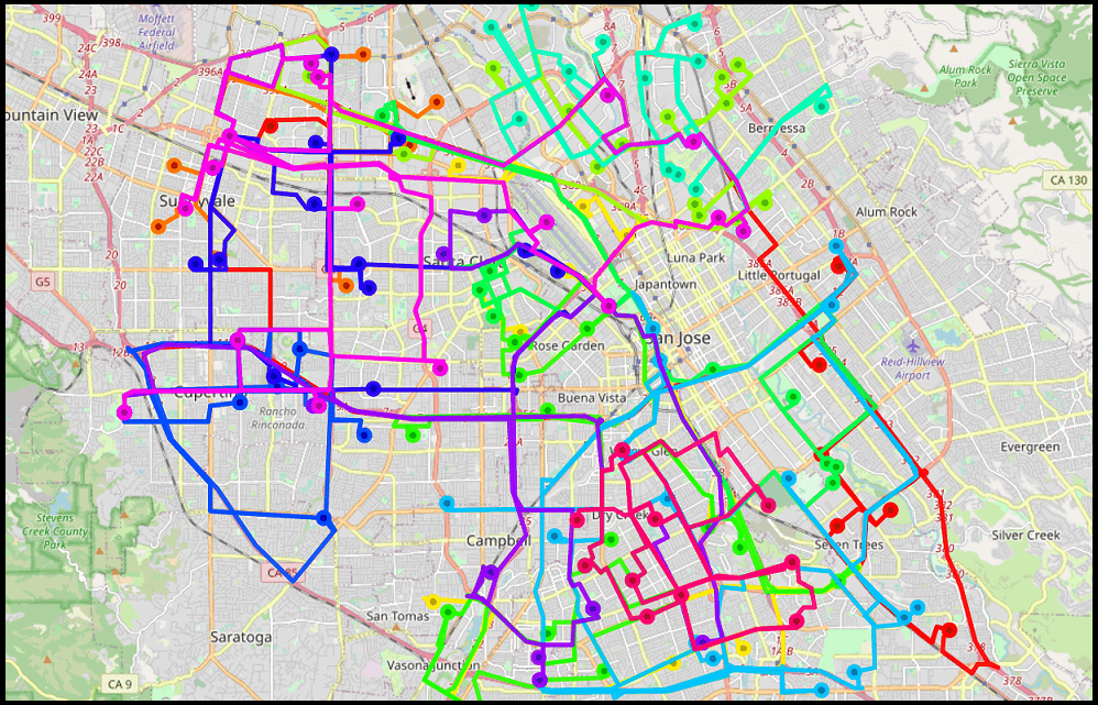
This model uses delay optimisation, on-board limits and pickup-delivery jobs. The following image shows output routes:

13.2 Next-day non-emergency patient transportation - soft rules
The following directory contains a non-realtime (i.e. next day) model for non-emergency patient transportation which uses soft rules (i.e. soft limits on time windows and onboard times):
supporting-data-for-docs\example-models\next-day-non-emergency-patient-transportation-soft-rulesIt uses the same input data as the hard rules model but instead it demonstrates soft rules, where if a rule is broken (i.e. dropoff too late, passenger on-board for too long), instead of the job remaining unassigned, the optimiser will still assign the job but will seek to minimise the rule violation. This is suitable for scenarios where you have a fixed number of drivers available and all jobs must be served, even if some are served late.
See the readme.html in the directory for more information.
13.3 Realtime pickup-delivery problems (multi-restaurant food deliveries example)
ODL Live can be configured for realtime optimised control of food delivery from multiple restaurants. This is a pickup-delivery problem, so each job has two stops. Typically your model would need to include several advanced modelling features:
Modelling degradation of food quality based on time on-board the vehicle. This is done using on-board time penalties.
Modelling customer (dis)satisfaction based on food delivery time. Customers would prefer their food ASAP but would typically only complain if they perceive their food to be ‘late’ - e.g. more than one hour. This creates a trade-off between routing efficiency and customer satisfaction. This is modelled using custom penalty functions on delivery time.
Modelling pickup time at restaurant when multiple orders are collected together. This is modelled using parking time, so we support logic like ‘include 10 minutes for first pickup at a restaurant and a further minute for each subsequent pickup’.
13.3.1 Job configuration
The following example JSON shows our recommended setup for hot food delivery jobs. The specific cost multipliers and times will need to be tuned to individual use cases but the structure of the job JSON (i.e. its fundamental rules) should not change:
{
  "quantities": [
    1
  ],
  "breakAllowedBetweenStops": false,
  "stops": [
    {
      "type": "SHIPMENT_PICKUP",
      "durationMillis": 60000,
      "coordinate": {
        "latitude": 40.70440673828125,
        "longitude": -74.00933074951172
      },
      "parking": {
        "parkingTimeSeconds": 120,
        "parkingTimeMinSeparationMetres": 1,
        "cost": 1
      },
      "multiTWs": [
        {
          "openTime": "2018-01-02T01:33",
          "closeTime": "2018-01-03T01:33",
          "penalties": [
            {
              "openTime": "2018-01-02T01:33",
              "costPerHour": 5,
              "join": "EXACT"
            },
            {
              "openTime": "2018-01-02T02:18",
              "costPerHour": 100,
              "costPerHourSqd": 100,
              "join": "EXACT"
            }
          ]
        }
      ],
      "_id": "P1"
    },
    {
      "type": "SHIPMENT_DELIVERY",
      "durationMillis": 180000,
      "coordinate": {
        "latitude": 40.73283004760742,
        "longitude": -74.0078125
      },
      "multiTWs": [
        {
          "openTime": "2018-01-02T01:33",
          "closeTime": "2018-01-03T01:33",
          "penalties": [
            {
              "openTime": "2018-01-02T01:33",
              "costPerHour": 5,
              "join": "EXACT"
            },
            {
              "openTime": "2018-01-02T02:18",
              "costPerHour": 100,
              "costPerHourSqd": 100,
              "join": "EXACT"
            }
          ]
        }
      ],
      "_id": "D1"
    }
  ],
  "onboardTimePenalty": {
    "type": "FROM_LEAVE_LOC",
    "hoursPenalty": [
      {
        "inclusiveLowerLimit": 0.25,
        "c1": 10,
        "join": "EXACT"
      },
      {
        "inclusiveLowerLimit": 0.5,
        "c0": 2.5,
        "c1": 1000,
        "c2": 1000,
        "join": "EXACT"
      }
    ]
  },
  "_id": "Job1"
}
Warning when you are modifying the JSON to set your own cost values, if you misspell a field, the field will usually be silently ignored by ODL Live instead of an error being reported. This is a design choice - if we remove a field from the API and the client sends us an old-format JSON still containing that field, we don’t break the system by rejecting that JSON. The way to check for typos when you’re doing system integration/testing is to GET the model after doing PUT and see if any of your fields are no longer present.
At the very top of our job JSON we have:
"quantities" : [ 1 ],quantities=1 says that the first quantity dimension for the job has a value of 1 unit. The unit only has meaning when we consider the vehicle - for example if the first quantity dimension for a vehicle is set to 3 then we can hold a maximum of 3 jobs on-board at once. We could have defined multiple quantities if we wanted, corresponding to limits like max on-board jobs, volume, weight etc. For example this following JSON defines the first two quantity dimensions instead:
"quantities" : [ 1 , 320],Next in the job JSON we have:
"breakAllowedBetweenStops" : falseThis is simple, if we’re modelling work breaks as well then we prevent the job being assigned such that the pickup is before the break and the delivery is after the break.
The structure of the job has two stops with two different coordinates and types SHIPMENT_PICKUP and SHIPMENT_DELIVERY respectively. The coordinate of the first stop is the restaurant and the second is the delivery location:
{
  "stops" : [ {
    "type" : "SHIPMENT_PICKUP",
    "coordinate" : {
      "latitude" : 40.70440673828125,
      "longitude" : -74.00933074951172
    },
    "_id" : "P1"
  }, {
    "type" : "SHIPMENT_DELIVERY",
    "coordinate" : {
      "latitude" : 40.73283004760742,
      "longitude" : -74.0078125
    },
    "_id" : "D1"
  } ],
  "_id" : "Job1"
}
The stop ids must be unique amongst all stops in the model.
13.3.1.1 Modelling pickup duration
The first stop specifies both (a) durationMillis which is a fixed time to service the stop and (b) a parking object which includes an additional ‘parking-related’ time:
{
    "type" : "SHIPMENT_PICKUP",
    "durationMillis" : 60000,
    "coordinate" : {
        ....
    },
    "parking" : {
      "parkingTimeSeconds" : 120.0,
      "parkingTimeMinSeparationMetres" : 1.0,
      "cost" : 1.0
    },
    "_id" : "P1"
}
The parking time and parking cost are applied when we arrive at the stop from another location which is further than parkingTimeMinSeparationMetres distant from the stop (in this case 1 metre). Multiple pickups at the same restaurant should have exactly the same latitude/longitude values and the same configuration for the parking object (e.g. same parkingTimeSeconds and cost). The first pickup of several consecutive pickups at a restaurant will have the parking time seconds and parking cost applied to it, but subsequent consecutive pickups (i.e. pickups at the same time) will not. durationMillis will still be applied to each pickup. Therefore given a route P1, P2, D1, D2 where the pickups P1 and P2 are at the same location, the total pickup time in seconds for all pickup stops should be:
The field parking.cost acts as a penalty which is applied when pickups at the same location are not served together. If you increase it, especially once it gets larger than the on-board penalty or delivery time penalties, you are more likely to group pickups at restaurants at the expense of being late or having the food on-board for too long. If multiple pickups are happening at once, you should ideally group the stop completion events for these pickups and send them in one update as a GPS trace update after one pickup stop completion event but before other pickup completion events could confuse the parking time logic.
13.3.1.2 Modelling delivery time preferences
We model delivery time dependence using the multiTWs object and custom lateness penalties. You are advised to read this section which describes the multiTWs object in-detail. We have exactly the same multiTWs structure defined for both the pickup and delivery stop. Technically for customer satisfaction we probably only care about the delivery time window and so could just place the delivery time penalty functions defined within multiTWs on the delivery stop only. However defining the penalties twice for both the pickup and delivery stops helps the optimiser to search more efficiently, as it will reject some potential pickup permutations earlier (i.e. defining these penalties twice speeds the optimiser up considerably and is strongly advised).
We look at this multiTWs structure in more detail:
"multiTWs" : [
    {
      "openTime": "2018-01-02T01:33",
      "closeTime": "2018-01-03T01:33",
      "penalties": [
        {
          "openTime": "2018-01-02T01:33",
          "costPerHour": 5,
          "join": "EXACT"
        },
        {
          "openTime": "2018-01-02T02:18",
          "costPerHour": 100,
          "costPerHourSqd": 100,
          "join": "EXACT"
        }
      ]
    }
  ]
This JSON defines a time window and a lateness penalty function (comprised of 2 subfunctions) within that time window. Within this JSON, multiTWs[0].openTime is the earliest the stop could be served, corresponding to earliest pickup at the restaurant (there’s no point picking up before the food is ready). This is only relevant for the pickup stop, but for simplicity we set it the same on both stops. The multiTWs[0].openTime and all other times in the job JSON are defined in UTC, not the local time zone where the deliveries are being done.
multiTWs[0].closeTime is a hard limit on the latest allowed arrival at a stop. We set an arbitrarily late closeTime (actually the openTime plus 24 hours). We don’t actually expect delivery to happen 24 hours late, instead we’re just turning off the hard limit by setting it far in the future and using the cost penalties to get the behaviour we want - i.e. penalising late deliveries to prevent them. Hard limits are generally a bad idea when running in realtime, as GPS updates etc could push the current plan repeatedly into and out of the hard limit violation, causing the job to be randomly unloaded and reloaded in the plan.
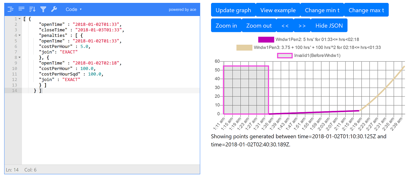
Following the instructions in the section on multi time windows and custom penalties we can view a graph of the lateness penalties defined in our multiTWs JSON:

We’ve setup the time penalties so we have:
A relatively small penalty that increases linearly with the estimated time of delivery is used, providing the estimated time of delivery is not considered ‘late’. This penalty is traded-off against route efficiency (total travel time) and the on-board time penalty. It encourages the optimiser to deliver the order early, but not if this means a lot more driving. This small penalty appears on the graph as the dark pink/purple line going from 1:33am to 2:18am.
A much larger penalty comes into effect if the estimated time of delivery is considered ‘late’. Providing the on-board time is not being significantly violated, this strongly encourages the optimiser to complete the order ASAP. The yellow-brown line from 2:18am onwards on the graph shows this larger penalty. If you zoom out some more on the graph using the zoom controls, you can see this penalty rises sharply.
The section on multi time windows contains an in-depth explanation of how these lateness penalty function are defined.
When running in realtime the optimiser will shift pre-dispatched jobs around between vehicles to minimise these cost functions - i.e. to minimise lateness - as much as is possible. You should continually monitor the current optimiser plan for significant predicted lateness, by checking the estimate arrival times at stops. If you do find significant lateness, this cannot be fixed by a clever assignment of jobs to vehicles (otherwise the optimiser would have done this already), and instead requires a manual intervention - i.e. human supervisor decides to cancel a job or give the customer a courtesy call to tell to apologise in-advance for their order being late. So in realtime we let ODL Live automatically control the dispatching and we only manually intervene on the odd occasion when issues arise that cannot be fixed by intelligent planning alone.
13.3.1.3 Modelling on-board time preferences
We have the following on-board time penalty defined:
"onboardTimePenalty" : {
    "type" : "FROM_LEAVE_LOC",
    "hoursPenalty" :  [ {
      "inclusiveLowerLimit" : 0.25,
      "c1" : 10.0,
      "join" : "EXACT"
    }, {
      "inclusiveLowerLimit" : 0.5,
      "c0" : 2.5,
      "c1" : 1000.0,
      "c2" : 1000.0,
      "join" : "EXACT"
    } ]
}
The section on on-board time penalties provides a detailed explanation of how on-board time penalties work. onboardTimePenalty.hoursPenalty is a penalty function, which are described in-detail in the section on penalty functions.
If you are using on-board time penalties, you may also need during-optimisation delays to minimise the on-board time, depending on how your stop time windows are setup. See this section for a detailed explanation.
In this example we are not using a hard limit and so we haven’t set the prohibited term. As with the delivery time penalty we recommend in a realtime setting you should not use a hard limit and instead monitor and manually intervene when you see a significant on-board time violation that cannot be fixed by the optimiser’s clever scheduling. Monitor on-board time by recording your ‘leave restaurant’ time and checking the estimated delivery time in the plan.
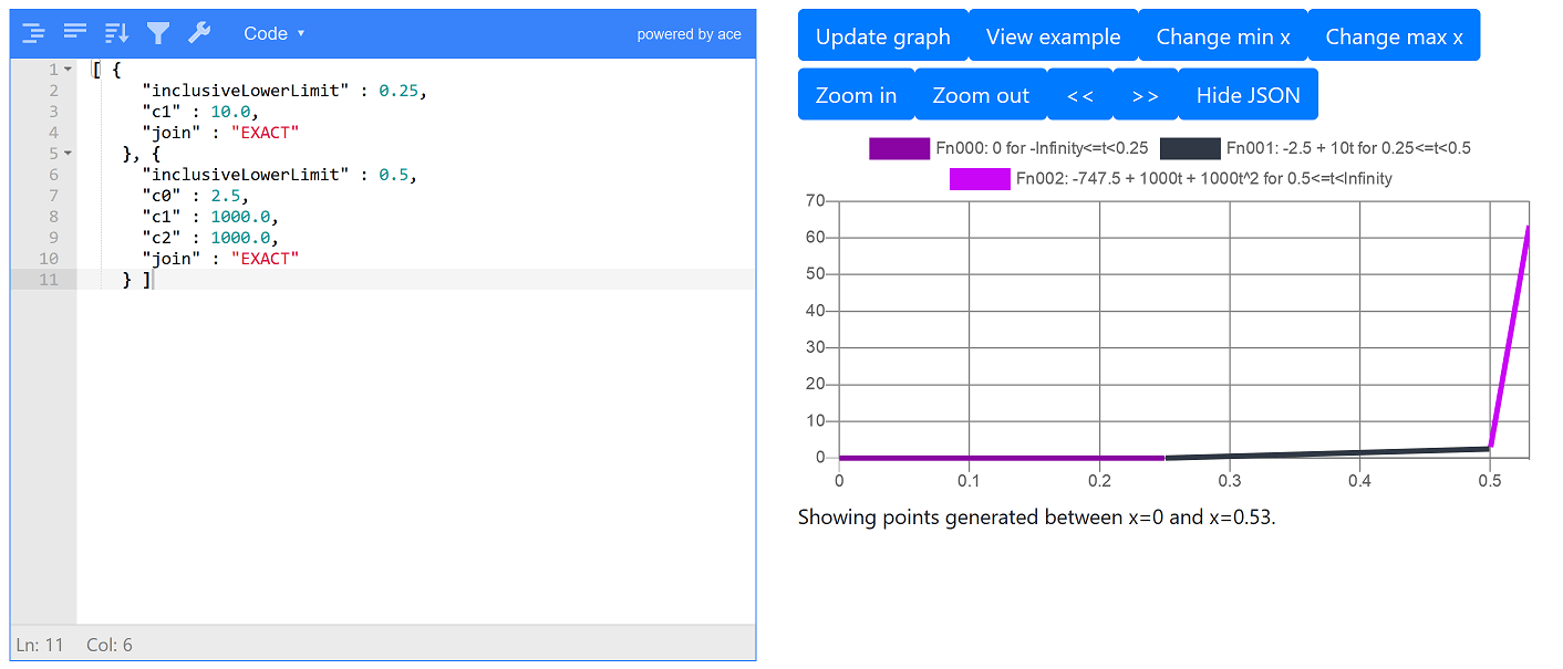
Following the instructions in the section on penalty functions, we use the penalty functions graph viewer to view our example on-board time penalty function:

We see the following:
No cost for the item being on-board less than 0.25 hours (i.e. 15 minutes). This is shown on the graph as the horizonal dark purple line at y = 0 between x = 0 and x = 0.25.
A modest penalty if the item is on-board less than half an hour (slightly sloped black line from x = 0.25 to x = 0.5).
A steeply rising penalty after half an hour (lighter purple line after x = 0.25).
The on-board time costs will be traded-off against the delivery time penalties and the travel cost (defined on the vehicle). Ideally you want your operations to run (i.e. have enough driver resource) such that both on-board penalty and delivery time penalty stay within the low-cost area (for the examples, on-board less than 30 minutes and delivery within 55 minutes of ordering). If either your estimated delivery time or estimated on-board time enters a high cost region, the optimiser will then try its best to get the value back down to a low cost region by moving jobs around.
13.3.2 Vehicle configuration
The following JSON defines a vehicle designed to work with the type of jobs defined in the previous section:
{
  "definition" : {
    "costPerTravelHour" : 1.0,
    "costPerWaitingHour" : 0.5,
    "costPerServicingHour" : 1.0,
    "costPerKm" : 1.0E-6,
    "costFixed" : 0.0,
    "costPerStop" : 0.0,
    "start" : {
      "type" : "START_AT_DEPOT",
      "coordinate" : {
        "latitude" : 40.75004577636719,
        "longitude" : -73.9950180053711
      },
      "openTime" : "2018-01-01T23:00",
      "_id" : "Start1"
    },
    "end" : {
      "type" : "RETURN_TO_DEPOT",
      "lateTime" : "2018-01-02T06:00",
      "closeTime" : "2018-01-02T23:00",
      "_id" : "End1"
    },
    "capacities" : [ 3 ]
  },
  "_id" : "V1"
}
costFixed is the cost for using the vehicle, regardless of the number of jobs assigned to it. We set costFixed = 0 as we assume we don’t want to minimise the number of vehicles used, because either (a) we’re paying vehicles by job or miles driven only or (b) we’ve already booked our drivers for the night and want to ensure they’re all used as much as possible.
costPerTravelHour and costPerServicingHour are both set to 1. These are the hourly costs for the driver doing work, either servicing an order or driving somewhere. It is assumed we want to minimise the driving time and hence we trade-off it off against both on-board time and delivery time, whilst these two metrics are in the ‘low cost’ region. You should ensure costPerTravelHour > 0 (i.e. it is never 0 or negative). You can set costPerTravelHour to be smaller than we’ve defined if wanted (e.g. 0.0001), but always greater than 0. You are advised to set costPerTravelHour to be several orders of magnitude larger than costPerKm as we want to prioritise reducing travel time over travel distance. If instead we prioritised reducing travel distance, the optimiser may order stops to encourage driving down short-but-direct back streets, instead of faster-but-less-direct highways.
We set costPerStop = 0 but if drivers are paid per job and different drivers have different per-job rates, you could model it here. Also if you find some vehicles are underused, or not used at-all, you could manipulate costPerStop over the delivery period, setting to smaller values for vehicles that have not had enough jobs dispatched to them and to larger values for vehicles that have had too many jobs dispatched to them. For example, you could set costPerStop proportional the average number of jobs a driver has had dispatched per hour, over the course of their shift so-far.
Vehicle start location and start time are defined in the start object. Then end object defines a lateTime when we would like the vehicle to finish by. By default the optimiser heavily penalises the vehicle finishing after its late time. We also define a hard end time (the closeTime field) but we set this to be many hours later (a day after the vehicle starts), again effectively turning off this hard limit. We have not set an end coordinate on the vehicle; setting one would encourage the assignment of jobs that take the vehicle back towards its base, which is probably not a beneficial strategy for realtime food delivery.
Vehicle capacity is set to 3, so 3 jobs can be held on-board at once. More capacity dimensions corresponding to weight, volume etc. could be added to this array if needed.
13.3.2.1 Updating the vehicle in realtime
The realtime planning walkthrough shows how to update a vehicle in real-time with GPS, dispatched, arrived and completed events. Assuming a vehicle is allowed to hold multiple orders at once you are advised to dispatch the pickup stops and delivery stops separately, to allow additional pickups to potentially be done after the dispatched pickup (this will only be done if it doesn’t increase the on-board time unacceptably anyway). So dispatch the pickup stop a few minutes before the vehicle needs to depart for the pickup location and dispatch the delivery stop a few minutes before the vehicle needs to depart for the delivery (e.g. when they’ve nearly arrived at the pickup location). In both cases, late dispatching is key; only dispatch stops shortly before the vehicle needs to start driving to them, to maximise the assignment options left open for the optimiser and therefore maximise the efficiency savings.
For completeness we show the JSON below of our recommend vehicle setup but with example realtime information attached:
{
  "definition" : {
    "costPerTravelHour" : 1.0,
    "costPerWaitingHour" : 0.5,
    "costPerServicingHour" : 1.0,
    "costPerKm" : 1.0E-6,
    "costFixed" : 0.0,
    "costPerStop" : 0.0,
    "start" : {
      "type" : "START_AT_DEPOT",
      "coordinate" : {
        "latitude" : 40.75004577636719,
        "longitude" : -73.9950180053711
      },
      "openTime" : "2018-01-01T23:00",
      "_id" : "Start1"
    },
    "end" : {
      "type" : "RETURN_TO_DEPOT",
      "lateTime" : "2018-01-02T06:00",
      "closeTime" : "2018-01-02T23:00",
      "_id" : "End1"
    },
    "capacities" : [ 3 ],
  },
  "dispatches" : [ {
    "creationTime" : "2018-01-01T23:11",
    "stopId" : "P6"
  }, {
    "creationTime" : "2018-01-01T23:21:49.942573405",
    "stopId" : "D6"
  }, {
    "creationTime" : "2018-01-01T23:40:40.817499473",
    "stopId" : "P79"
  }, {
    "creationTime" : "2018-01-01T23:48:13.056",
    "stopId" : "P216"
  }, {
    "creationTime" : "2018-01-01T23:49:13.591615601",
    "stopId" : "D216"
  }, {
    "creationTime" : "2018-01-01T23:56:53.103233787",
    "stopId" : "D79",
  } ],
  "stopArrivedEvents" : [ {
    "time" : "2018-01-01T23:21",
    "stopId" : "P6",
    "_id" : "TZ60kJG6RuOEVvA_NAnw-A=="
  }, {
    "time" : "2018-01-01T23:45:36.178573405",
    "stopId" : "D6",
    "_id" : "mOfcVsbERpq31egRKhQWUQ=="
  }, {
    "time" : "2018-01-01T23:57:18.986499473",
    "stopId" : "P79",
    "_id" : "XfO6P70dQ_q4dMnWBAx_MQ=="
  }, {
    "time" : "2018-01-01T23:58:13.056",
    "stopId" : "P216",
    "_id" : "kw9m_mDhQFCG-svC66bipg=="
  } ],
  "stopCompleteEvents" : [ {
    "time" : "2018-01-01T23:32",
    "stopId" : "P6",
    "_id" : "7AeJ3hCCQsWAhhquXYkUFA=="
  }, {
    "time" : "2018-01-01T23:48:36.178573405",
    "stopId" : "D6",
    "_id" : "miuff0hSR-iAFQjpmEpepQ=="
  }, {
    "time" : "2018-01-01T23:58:18.986499473",
    "stopId" : "P79",
    "_id" : "0FlufjHTSJeQlQvftdlfDA=="
  }, {
    "time" : "2018-01-01T23:59:13.056",
    "stopId" : "P216",
    "_id" : "GQe6rqSZSUWzK_QMFsrgEg=="
  } ],
  "vehicleTraceEvents" : [ {
    "time" : "2018-01-01T23:59:13.056",
    "coordinate" : {
      "latitude" : 40.73527908325195,
      "longitude" : -73.9853515625
    },
    "type" : "GPS_DEVICE",
    "_id" : "obDZ-0OlRqKtfN9qBdNRew=="
  } ],
  "_id" : "V1"
}
The ids on the arrival, completion and vehicle trace events are just randomly generated universally unique identifiers - use your own ids as you wish.
The vehicleTraceEvents should only contain one element - the last GPS event. Earlier GPS events would not be used.
13.3.3 Model configuration
The following JSON shows an example model - without any jobs or vehicles - but with the configuration fields that will be of-interest to this use case.
{
  "data" : {
    "jobs" : [ ],
    "vehicles" : [ ]
  },
  "configuration" : {
    "distances" : {
      "graphDirectory" : "C:\\path_to_road_network_graph",
      "roadNetworkTimeMultiplier" : 1.0,
      "useRoadNetwork" : true,
      "learnerFilename" : "C:\\path_to_traffic_learner_model\\nyclearnedmodel"
    },
    "timeOverride" : {
      "override" : "2018-01-01T23:00",
      "overrideType" : "SCHEDULER"
    }
  }
}
You should set the graphDirectory field, which is the path to your road network graph (see chapters on this) and if you’re using the traffic learner, also set learnerFilename field, which is the learner model file location. If you want to slow down speeds provided by the traffic learner, you can set roadNetworkTimeMultiplier > 1. The field useRoadNetwork should be true and when using the learner. If you don’t have the data available to build a traffic learner model, you could use ODL Live’s standard car speeds instead, which adjust for rush hours.
The timeOverride object is useful for testing, at it overrides the current time the optimiser uses for its calculations. You should never include this object when running in realtime though or the optimiser calculations will use the wrong current time. See the section on time override for more details.
13.3.4 Example mid-period snapshot model
The ‘supporting data for docs’ directory which comes with the self-hosting ODL Live version contains a subdirectory example-models\food-deliveries-from-restaurants for this chapter. It has the following files:
nycFoodDeliveriesSnapshot.json - a JSON file containing a mid-delivery period snapshot of the food deliveries model setup in New York, as described in this chapter. The time override is set in this snapshot to the simulated time when the snapshot was taken.
nycsubset-cutout-road-network-graph.zip - a zipped road network graph directory containing an area cut around New York suitable for running this JSON snapshot model. You should unzip this to a directory on your computer and then change the field configuration.distances.graphDirectory in the model JSON to point towards this directory, remembering directory separators in JSON require \\ not \.
learnedmodel - traffic learner built model, for this New York example. Save it to your computer and update the field configuration.distances.learnerFilename to point towards it, remembering \\ instead of \.
Once you’ve modified the JSON you can PUT the model to a locally-running ODL Live and examine the routes for the currently-planned stops in the dashboard.
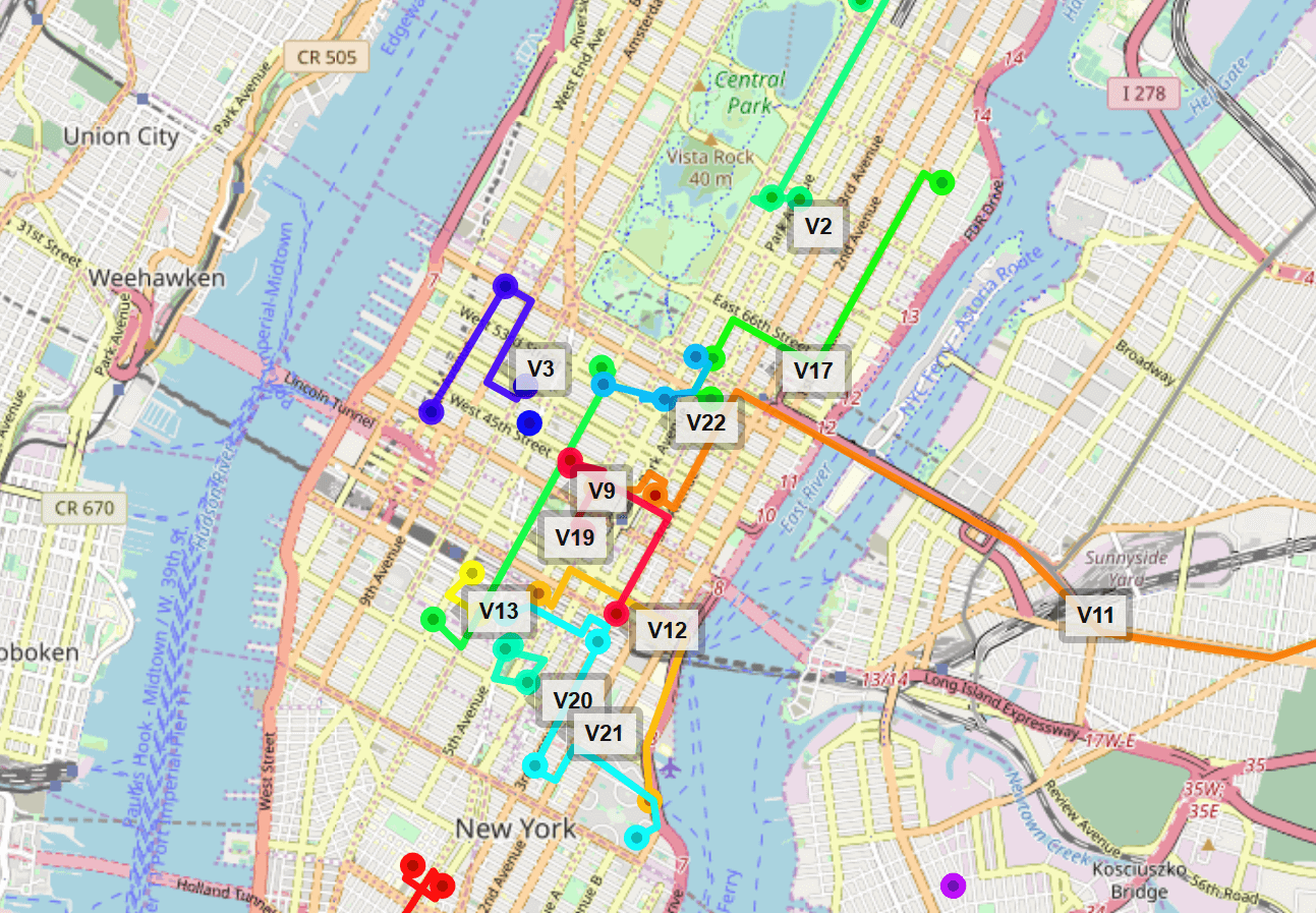
The following image shows some of the routes, where we’ve added the parameter ?noseq=true to the map URL to hide the sequence labels:

Note that when routes appear to not follow the roads exactly, this is because the road network geometry is being simplified a little when sent to your browser, to reduce data transfer. Internally the routes are modelled exactly on the roads.
There is also another (much simpler) example model demonstrating pickup-delivery jobs, onboard time limits, custom lateness penalties and delay optimisation in the following directory:
supporting-data-for-docs\example-models\simple-pd-with-soft-onboard-limits-and-delay-optimisation